Benchmarking {SpeedyMarkov}
Sam Abbott
2019-12-11
Source:vignettes/benchmarking.Rmd
benchmarking.RmdBenchmarking setup
The SpeedyMarkov and reference implementations have been benchmarked with a range of optimisations including making use of Rcpp and parallisation. Several parallisation approaches have been explored as has the use of a varying number of cores. The benchmarking grid has been implemented within SpeedyMarkov - see below for details.
- Load required packages.
library(SpeedyMarkov)
library(microbenchmark)
library(parallel)
library(furrr)
#> Loading required package: future
library(ggplot2)- Code for the benchmarking grid.
SpeedyMarkov::benchmark_markov
#> function (markov_model = NULL, reference = NULL, duration = NULL,
#>     samples = NULL, times = 1)
#> {
#>     future::plan(future::multiprocess, workers = 4)
#>     benchmark <- microbenchmark::microbenchmark(Reference = {
#>         reference(cycles = duration, samples = samples)
#>     }, R = {
#>         markov_ce_pipeline(markov_model(), duration = duration,
#>             samples = samples, sim_type = "base", sample_type = "base")
#>     }, `Rcpp inner loop` = {
#>         markov_ce_pipeline(markov_model(), duration = duration,
#>             samples = samples, sim_type = "armadillo_inner",
#>             sample_type = "base")
#>     }, `Rcpp simulation` = {
#>         markov_ce_pipeline(markov_model(), duration = duration,
#>             samples = samples, sim_type = "armadillo_all", sample_type = "base")
#>     }, `Rcpp simulation + sampling` = {
#>         markov_ce_pipeline(markov_model(), duration = duration,
#>             samples = samples, sim_type = "armadillo_all", sample_type = "rcpp")
#>     }, `Rcpp simulation + sampling - mclapply (2 cores)` = {
#>         markov_ce_pipeline(markov_model(), duration = duration,
#>             samples = samples, sim_type = "armadillo_all", sample_type = "rcpp",
#>             batches = 2, batch_fn = parallel::mclapply, mc.cores = 2)
#>     }, `Rcpp simulation + sampling - mclapply (4 cores)` = {
#>         markov_ce_pipeline(markov_model(), duration = duration,
#>             samples = samples, sim_type = "armadillo_all", sample_type = "rcpp",
#>             batches = 4, batch_fn = parallel::mclapply, mc.cores = 4)
#>     }, `Rcpp simulation + sampling - furrr::future_map (4 cores)` = {
#>         markov_ce_pipeline(markov_model(), duration = duration,
#>             samples = samples, sim_type = "armadillo_all", sample_type = "rcpp",
#>             batches = 4, batch_fn = furrr::future_map)
#>     }, times = times)
#>     return(benchmark)
#> }
#> <bytecode: 0x69e1e48>
#> <environment: namespace:SpeedyMarkov>
All benchmarking results have been run elsewhere (inst/scripts/benchmarking.R) and then saved (inst/benchmarks). These benchmarks can be recreated locally by running the following in the package directory (Warning:: This is likely to take upwards of an hour and a half).
Two state Markov model
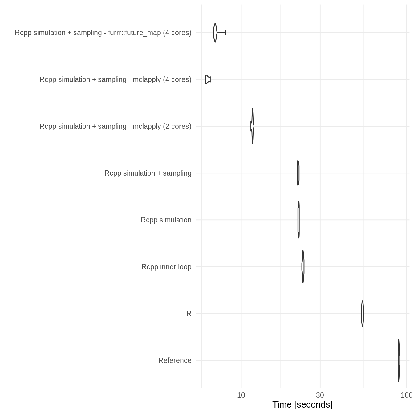
The two state Markov model has been benchmarked for both 100 cycles and 200 cycles (duration) with 100,000 samples each time - repeated 10 times per benchmark.
Benchmarking results show that both Rcpp implementations consistently outperform other implementations with the full Rcpp implementation being overall slightly faster but with potentially some instability. Parallisation appears to work well and scale with the number of cores used. Both parallisation approaches work equally well with furrr preferred due to its support for Windows. On a 4 core machine a parallel approach takes around 10% of the reference approaches runtime. There was also a substantial speed up - though less dramatic - when compared to the R SpeedyMarkov approach.
Increasing the number of cycles (duration) resulted in a an approximate doubling of the runtime for both the reference and R SpeedyMarkov approaches. However, all C++ based approaches had only small increases in runtime highlighting the increased performance that C provides (though the difference between the partial and full C++ approaches did increase). In fact the parallel C++ implementations showed no apparent increase in runtime when the duration was doubled. This indicates that this approach should scale well to more complex models and/or longer runtimes.
Duration: 100
- Table
two_state_bench_dur_100 <- readRDS("../inst/benchmarks/two_state_duration_100.rds")

two_state_bench_dur_100
#> Unit: seconds
#>                                                      expr       min        lq
#>                                                 Reference 45.583892 45.635655
#>                                                         R 30.400446 31.741273
#>                                           Rcpp inner loop 16.769725 16.886614
#>                                           Rcpp simulation 15.131577 15.420805
#>                                Rcpp simulation + sampling 14.827075 15.004812
#>           Rcpp simulation + sampling - mclapply (2 cores)  7.918256  8.103257
#>           Rcpp simulation + sampling - mclapply (4 cores)  4.186299  4.353983
#>  Rcpp simulation + sampling - furrr::future_map (4 cores)  4.934897  5.025115
#>       mean    median        uq       max neval
#>  45.904836 45.836815 46.083414 46.584301    10
#>  31.809249 31.794831 32.131458 32.525617    10
#>  17.089844 17.066265 17.242150 17.590342    10
#>  15.507085 15.455598 15.705200 15.820355    10
#>  15.212322 15.159396 15.312806 16.059966    10
#>   8.213000  8.136523  8.355903  8.579321    10
#>   4.543794  4.566942  4.713321  4.895079    10
#> 5.241085 5.080382 5.193253 6.657297 10- Plot
ggplot2::autoplot(two_state_bench_dur_100) +
  theme_minimal()
#> Coordinate system already present. Adding new coordinate system, which will replace the existing one.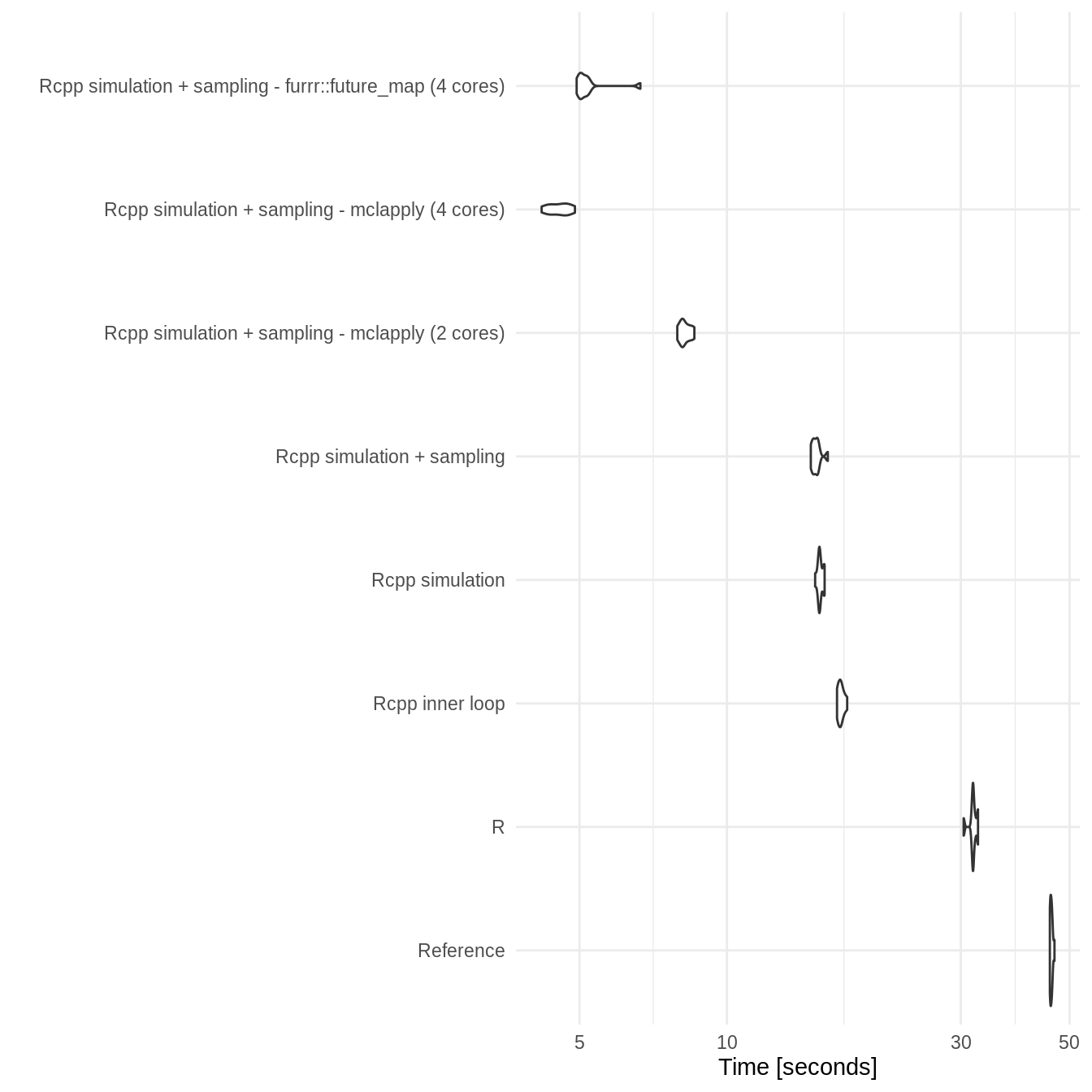
Duration: 200
- Table
two_state_bench_dur_200 <- readRDS("../inst/benchmarks/two_state_duration_200.rds")

two_state_bench_dur_200
#> Unit: seconds
#>                                                      expr       min        lq
#>                                                 Reference 88.771567 89.263467
#>                                                         R 53.205902 53.749978
#>                                           Rcpp inner loop 23.264311 23.551238
#>                                           Rcpp simulation 22.027613 22.065004
#>                                Rcpp simulation + sampling 21.793681 21.882913
#>           Rcpp simulation + sampling - mclapply (2 cores) 11.446995 11.648192
#>           Rcpp simulation + sampling - mclapply (4 cores)  6.074584  6.093671
#>  Rcpp simulation + sampling - furrr::future_map (4 cores)  6.827251  6.896384
#>       mean    median        uq       max neval
#>  89.603412 89.478862 89.995928 90.806615    10
#>  54.039097 54.062900 54.423413 54.874361    10
#>  23.651559 23.634217 23.824933 23.963772    10
#>  22.231128 22.253064 22.377521 22.409554    10
#>  22.060673 22.054814 22.229017 22.364376    10
#>  11.689546 11.693031 11.744444 11.938786    10
#>   6.276848  6.208936  6.535311  6.559263    10
#> 7.064807 6.970516 7.027639 8.075195 10- Plot
ggplot2::autoplot(two_state_bench_dur_200) +
  theme_minimal()
#> Coordinate system already present. Adding new coordinate system, which will replace the existing one.