Data exploration

Overview

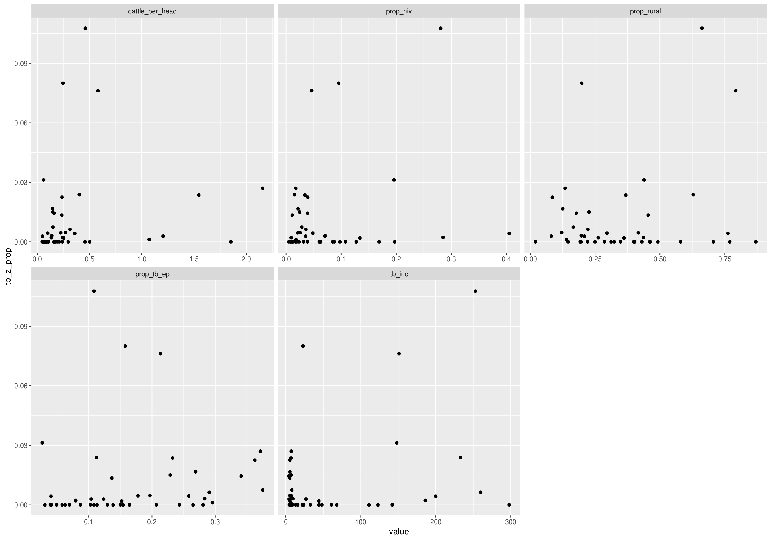
In this vignette the lastest data for the proportion of TB cases that are zoonotic, along with data on potential correlates, is rapidly explored using an EDA approach modelled on that used in the {DataExplorer} package. This analysis is indicative only and any findings should be evaluated more carefully using more robust techniques.

Data

Latest data available used by default - see data sources and data linkage for details. To instead explore the complete dataset comment out the get_latest_combined_data call and rerun the analysis.

This step also drops variables that are unlikely to be of interest in an initial EDA. This includes: confidence intervals, standard error, country names, country codes, and regions. On top of this countries with fewer than 100 TB cases have been removed, along with countries with incidence rates below 1 per 100,000 population (effective TB elimination). This has been done as data for these countries is unlikely to provide meaningful insights for a global model of zoonotic TB incidence.

latest_data <- link_data(verbose = FALSE) %>% 
  get_latest_combined_data() %>% 
  dplyr::filter(tb_cases > 100, tb_inc > 1) %>% 
  dplyr::select(-z_tb_study_pop, -contains("_lo"), -tb_inc_hi, -prop_hiv_hi, 
                -tb_z_prop_hi, -tb_z_prop_se, -country, -country_code, -g_whoregion)

Summary

Data table summary

knitr::kable(t(DataExplorer::introduce(latest_data)), 
             row.names = TRUE, 
             col.names = "", 
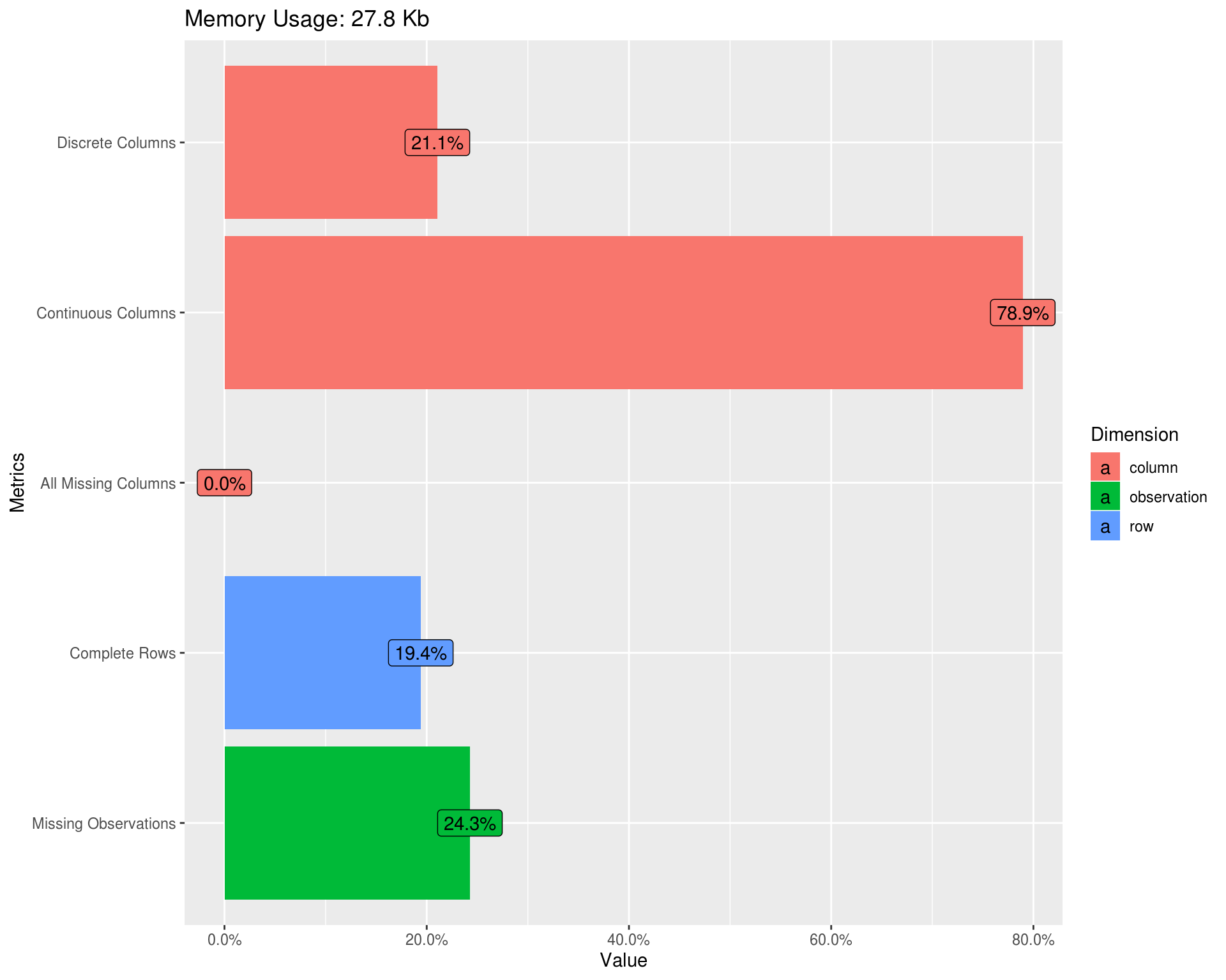
             format.args = list(big.mark = ","))

rows	170
columns	19
discrete_columns	4
continuous_columns	15
all_missing_columns	0
total_missing_values	784
complete_rows	33
total_observations	3,230
memory_usage	28,488

Data figure summary

DataExplorer::plot_intro(latest_data)

Missing values

DataExplorer::plot_missing(latest_data, geom_label_args = list(size = 3, label.padding = unit(0.1, "lines")))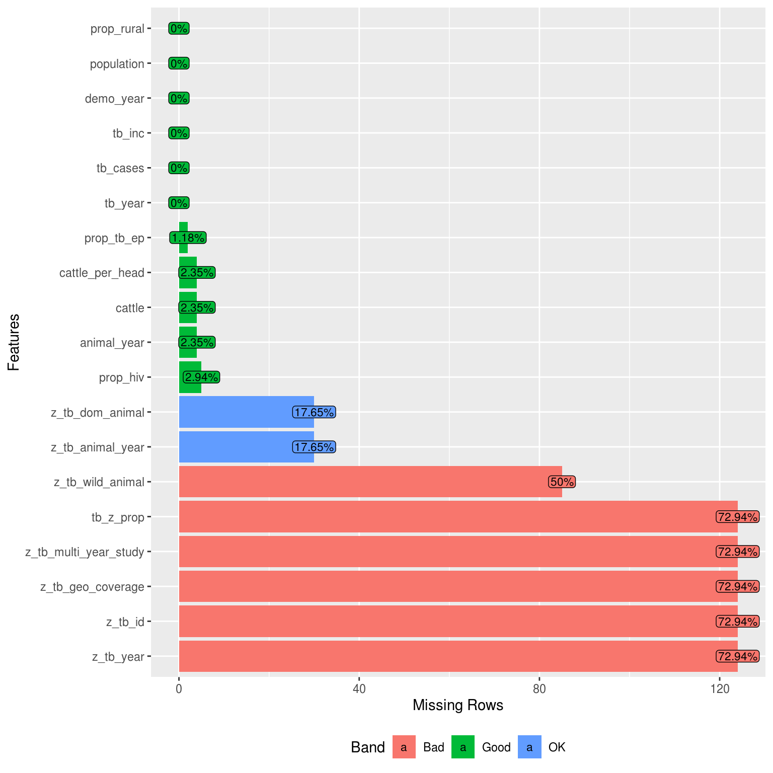

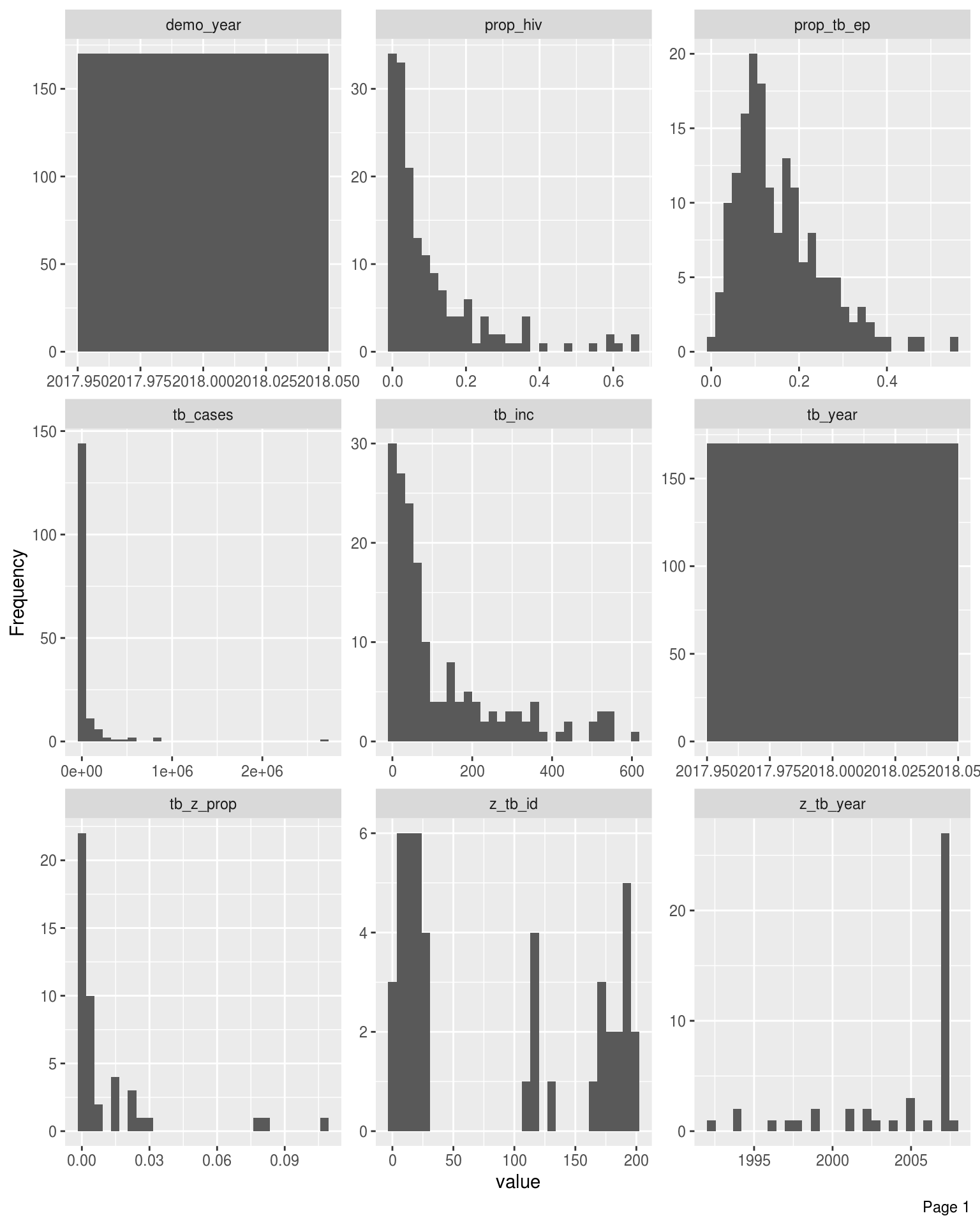
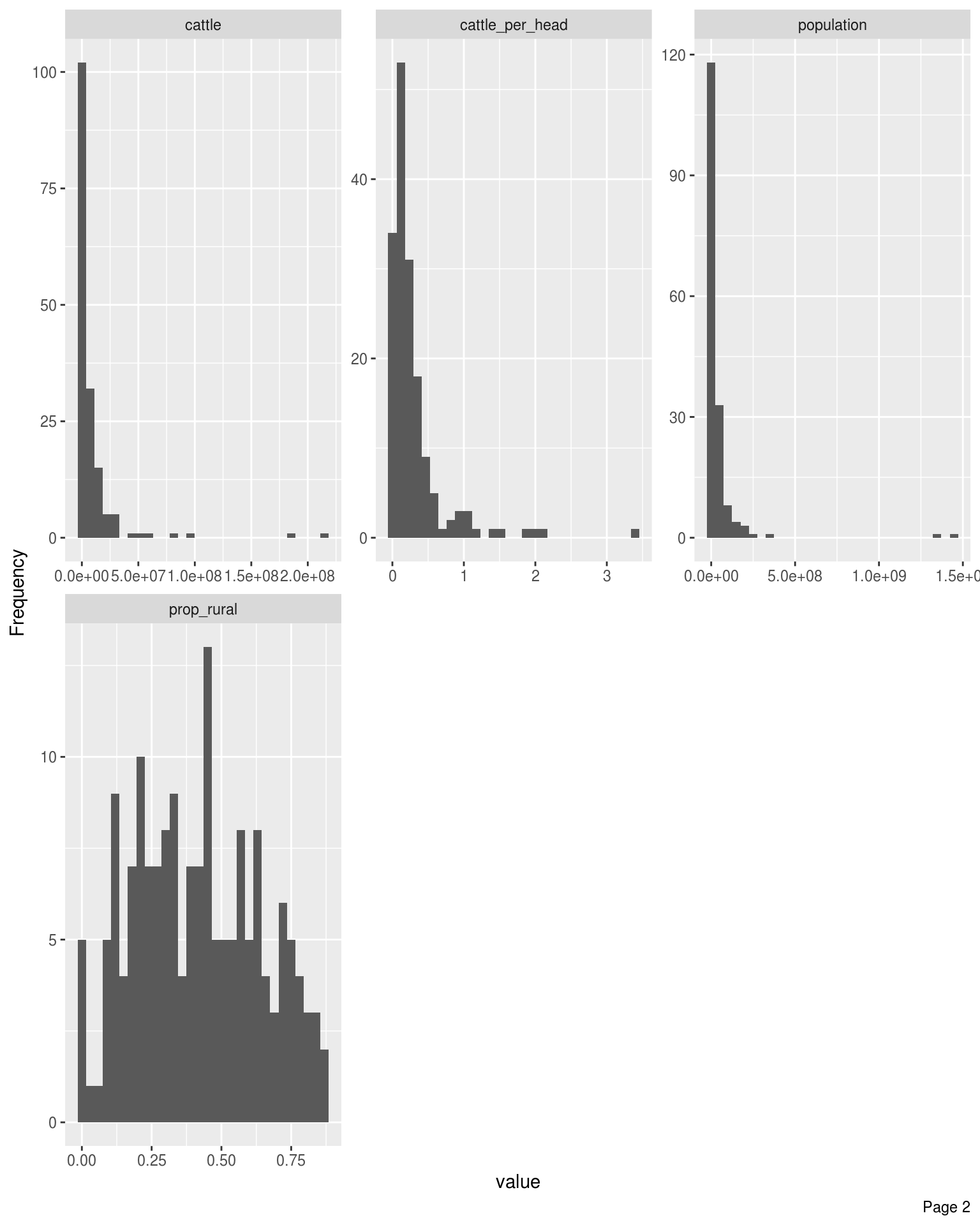
Distributions

Bar Charts

Frequency distributions for all discrete features

DataExplorer::plot_bar(latest_data, theme_config = list("text" = element_text(size = 12)), nrow = 4L, ncol = 3L)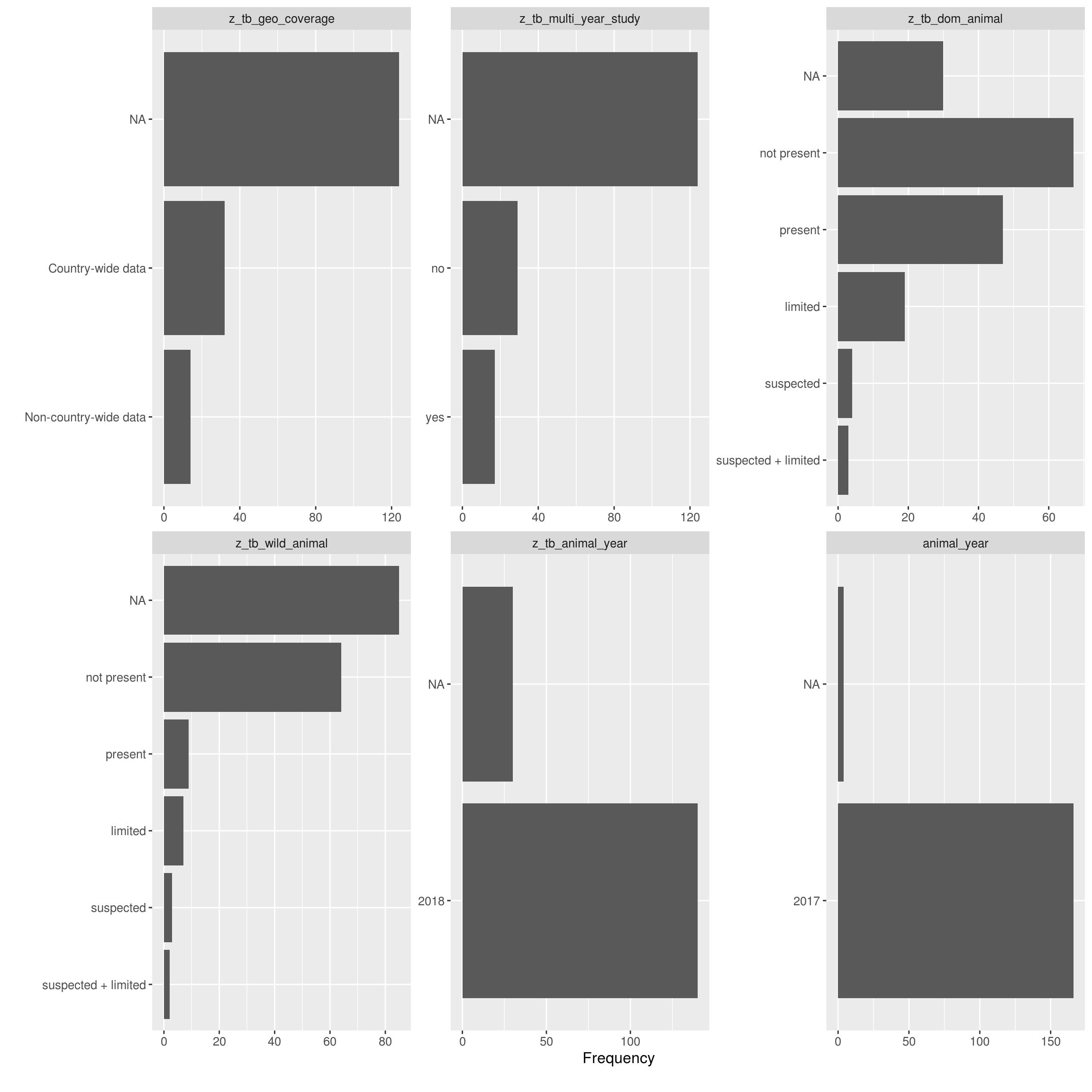

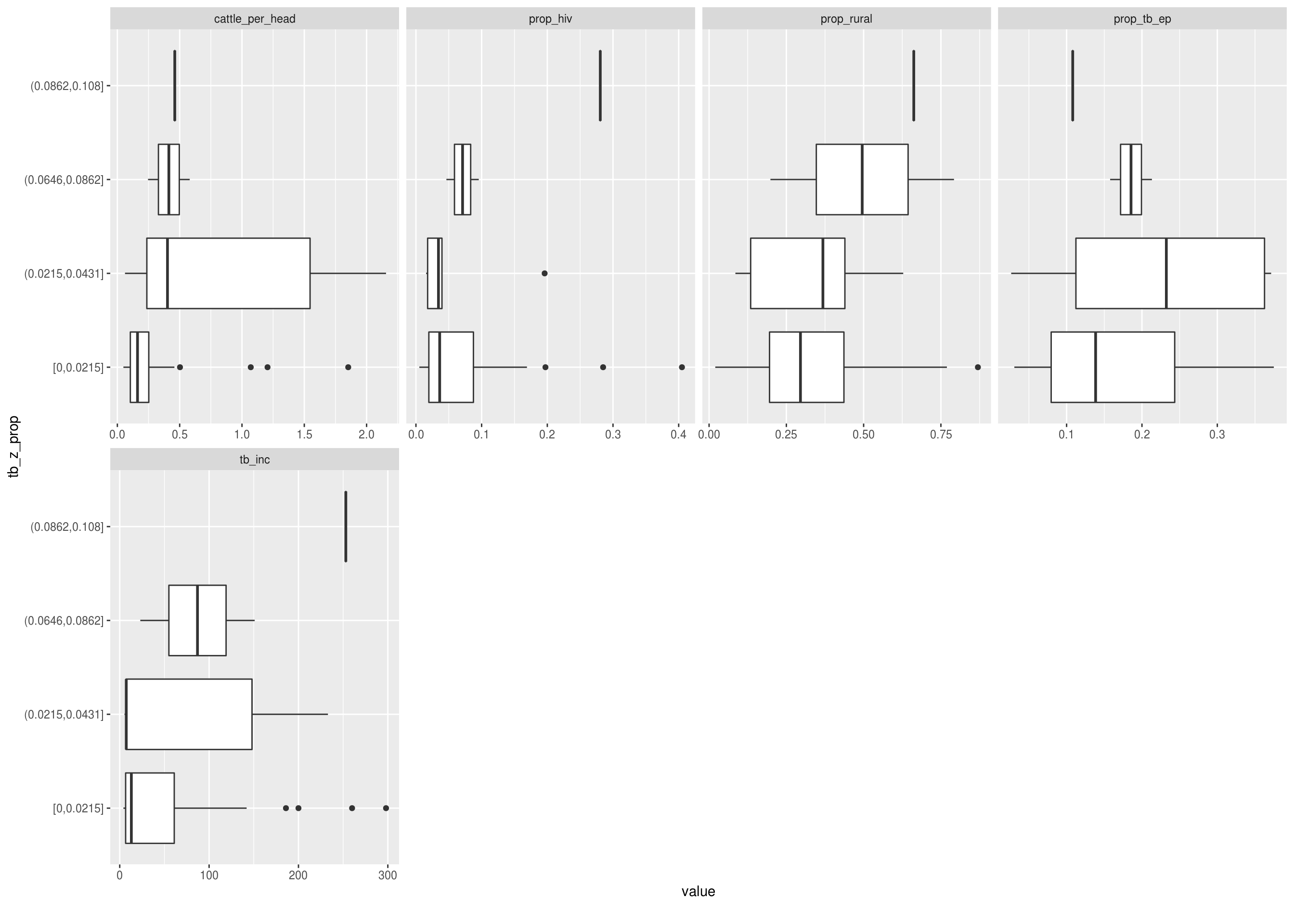
Discrete features by the proportion of TB cases that have zoonotic TB

DataExplorer::plot_bar(latest_data, with = "tb_z_prop", theme_config = list("text" = element_text(size = 12)))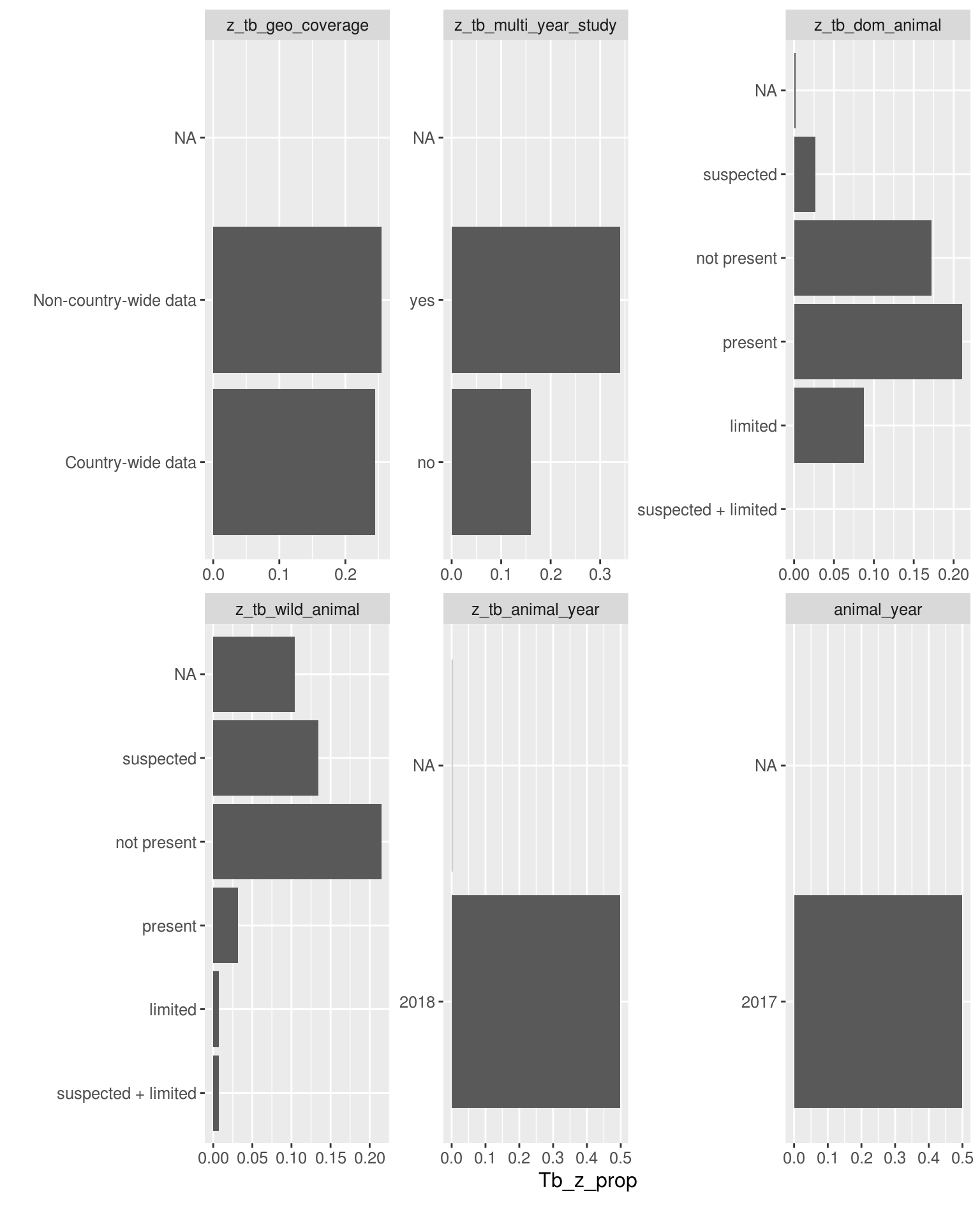

Histograms

Visualize distributions for all continuous features

suppressWarnings(DataExplorer::plot_histogram(latest_data, nrow = 3L, ncol = 3L))

Correlation Analysis

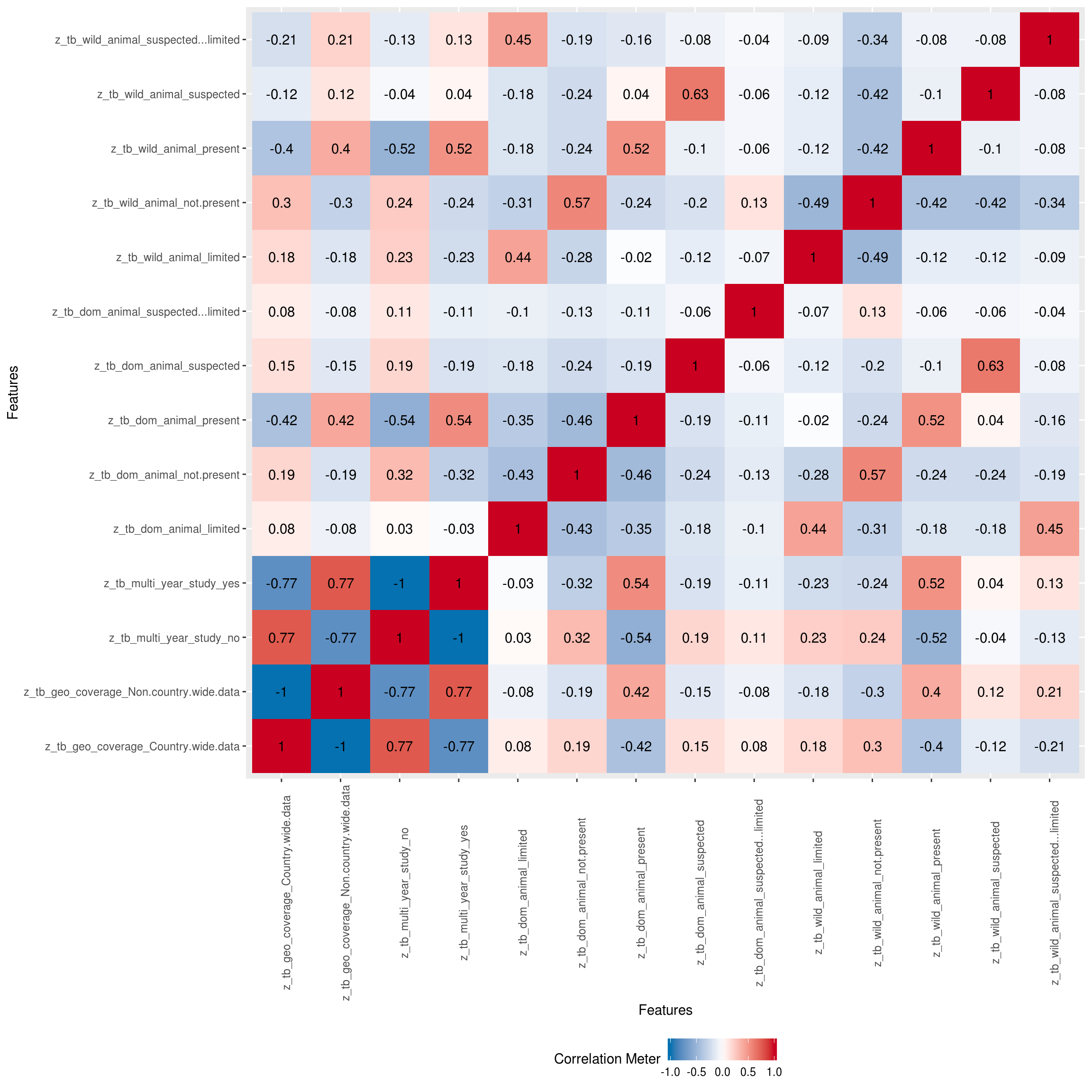
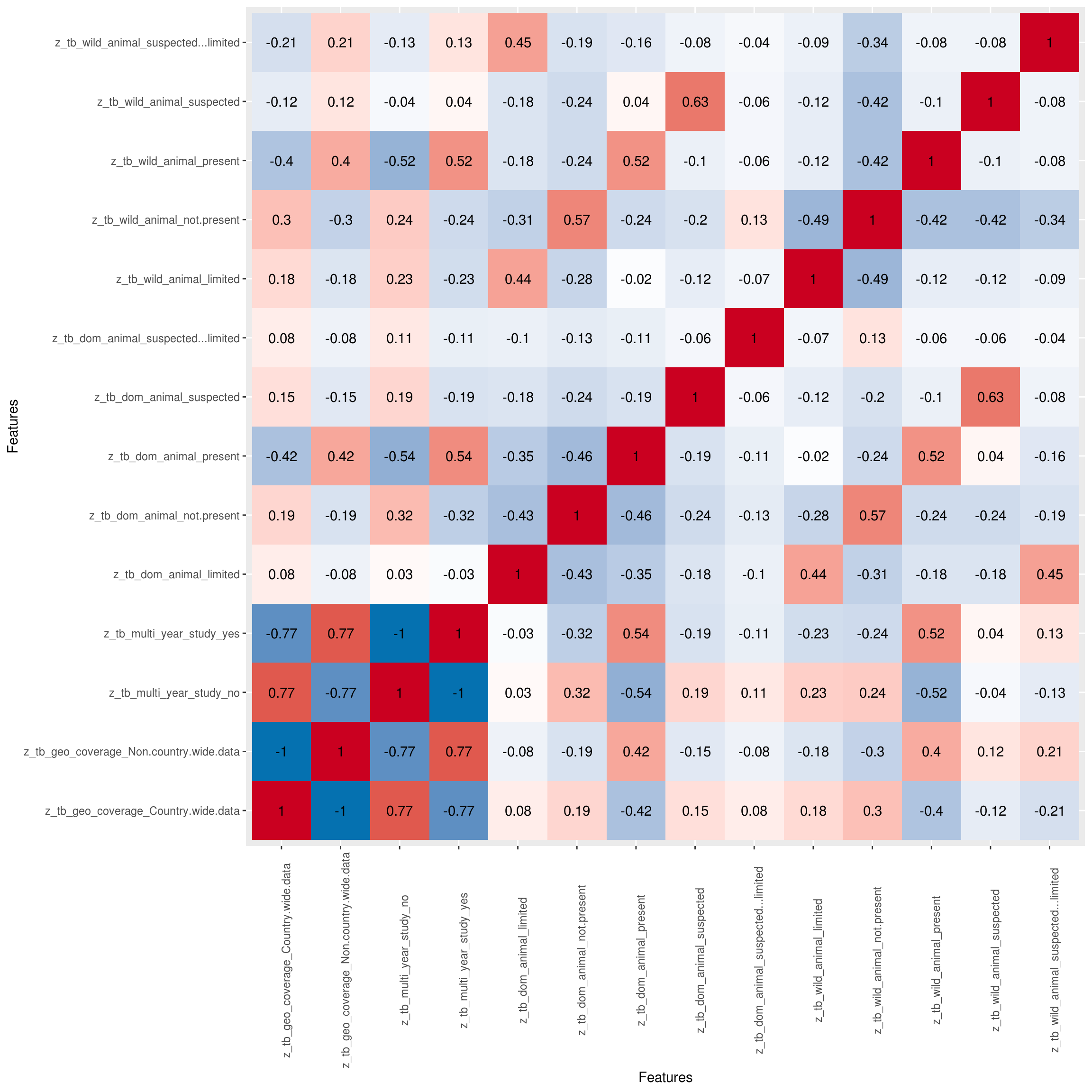
Visualize correlation heatmap for all non-missing features

DataExplorer::plot_correlation(na.omit(latest_data), maxcat = 5L)

## Warning in cor(x = structure(list(tb_year = c(2018, 2018, 2018, 2018,
## 2018, : the standard deviation is zero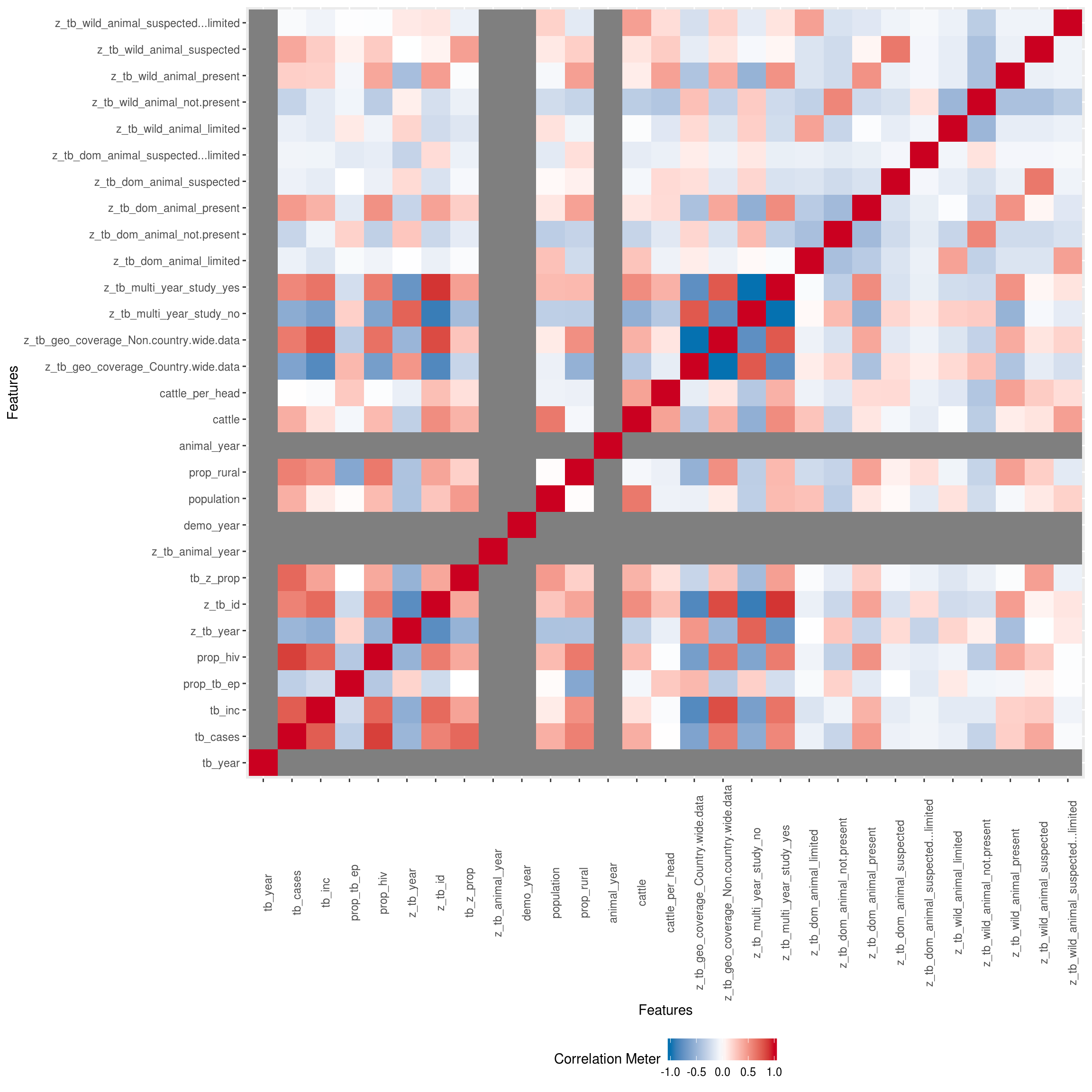

Only continuous features

plot <- DataExplorer::plot_correlation(na.omit(latest_data), type = "c") +
  theme(legend.position = "none")

## Warning in cor(x = structure(list(tb_year = c(2018, 2018, 2018, 2018,
## 2018, : the standard deviation is zero

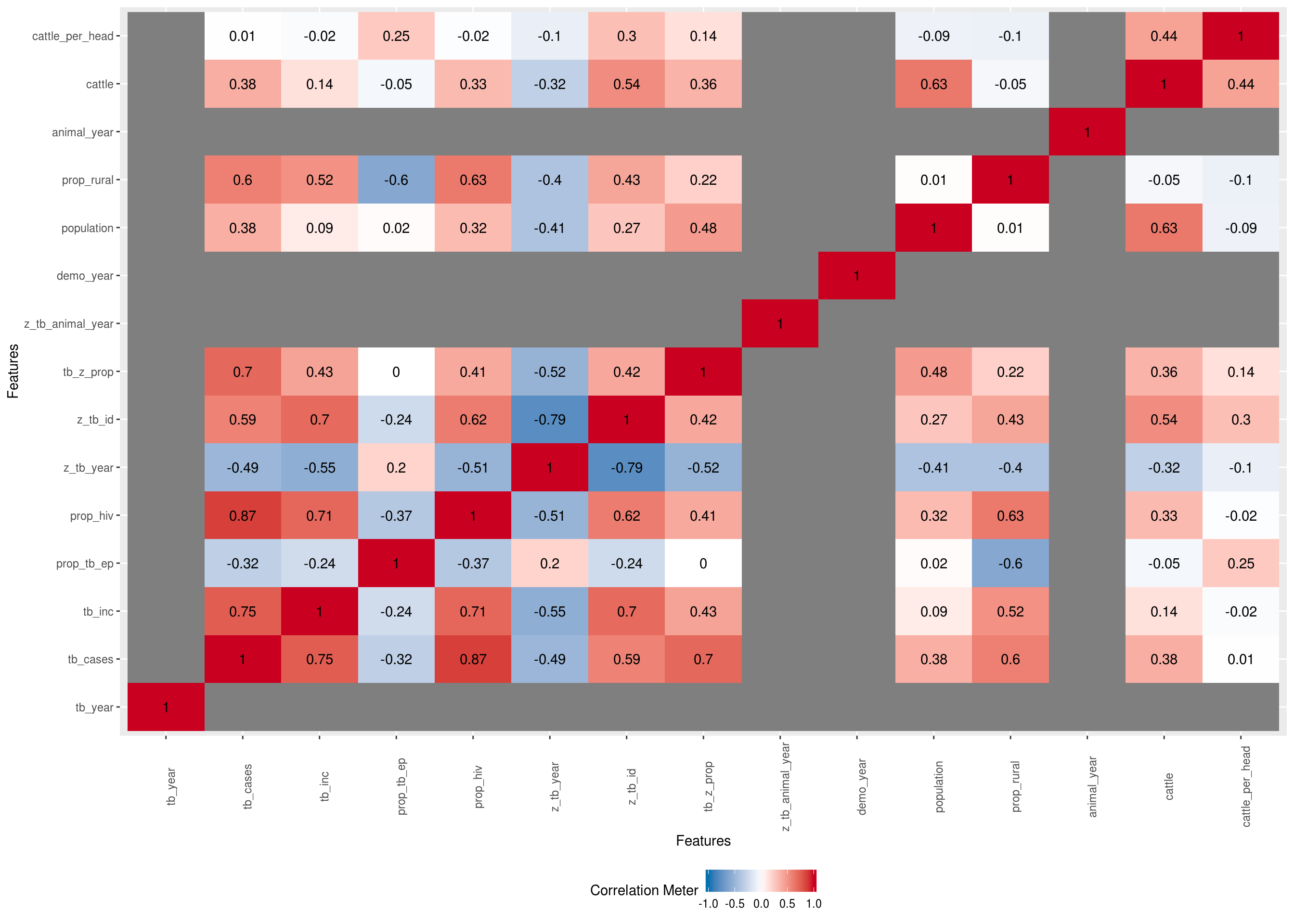
## Warning: Removed 100 rows containing missing values (geom_text).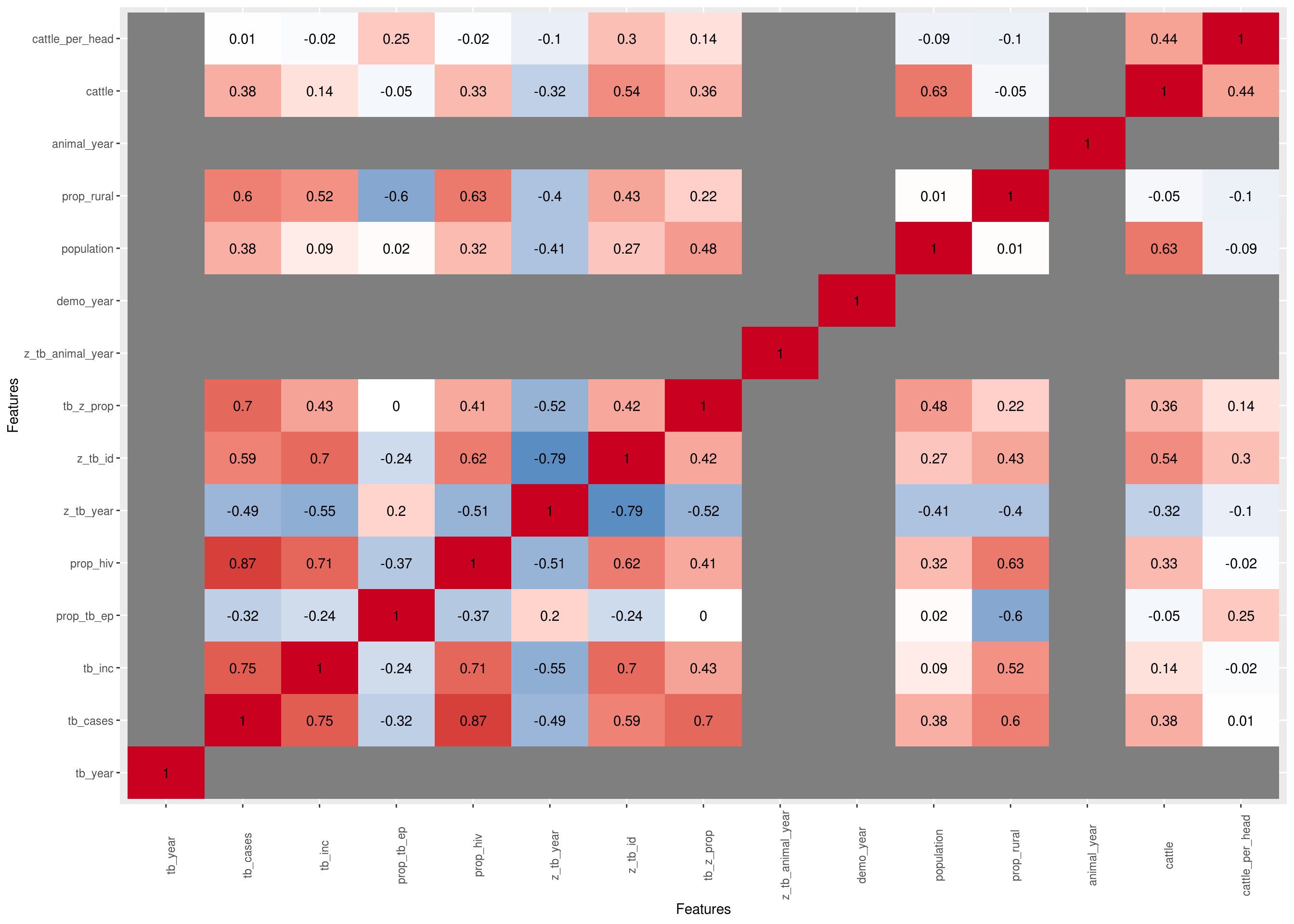

plot

## Warning: Removed 100 rows containing missing values (geom_text).

Only discrete features

DataExplorer::plot_correlation(na.omit(latest_data), type = "d") +
  theme(legend.position = "none")

Principal Component Analysis

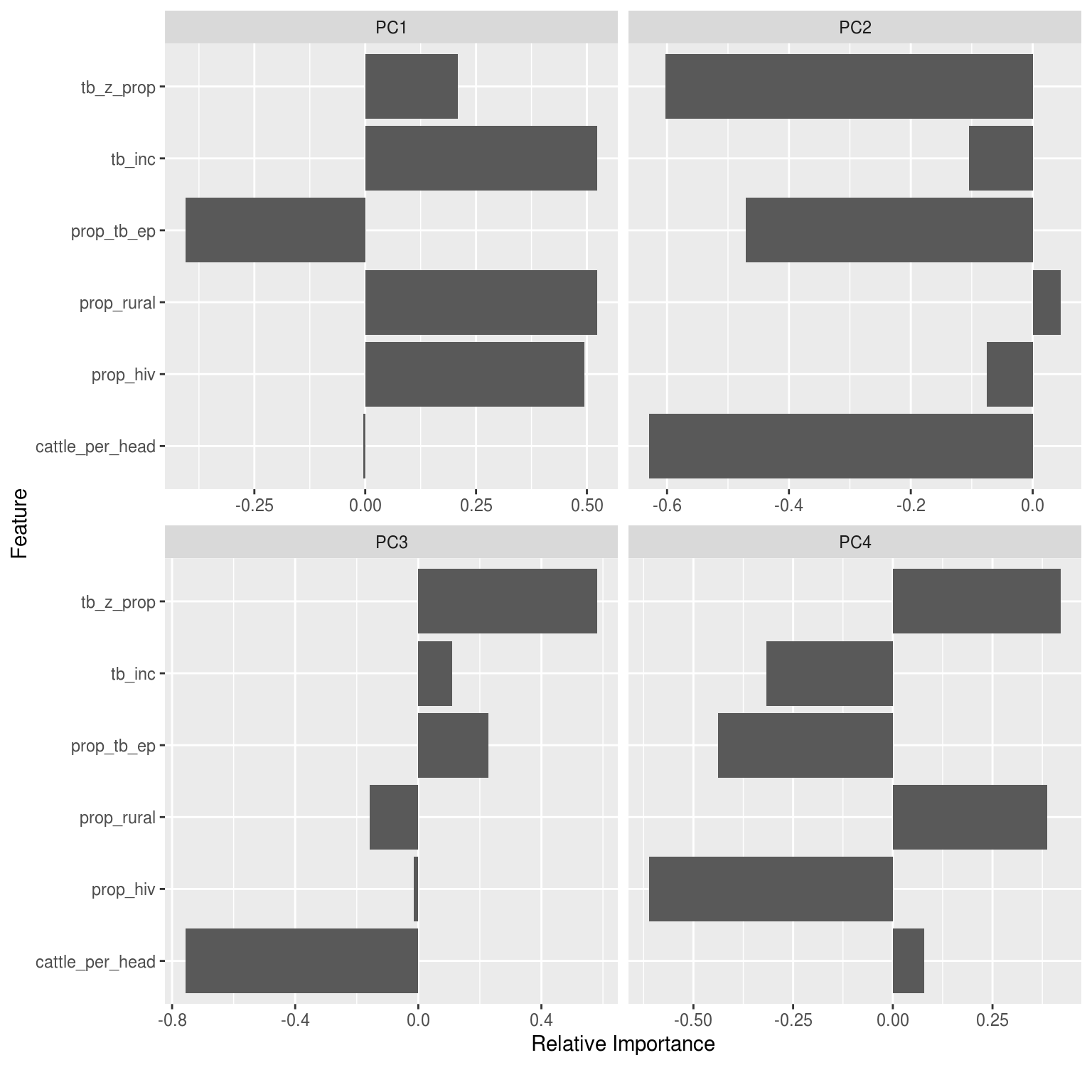
Drop all factor based variables, as well as time variables and raw incidence variables (as all just correlates of population).

pca_df <- latest_data %>% 
  dplyr::select(-contains("year"), -population, -tb_cases, -z_tb_id,
                -population, -cattle, -z_tb_geo_coverage, -z_tb_wild_animal, 
                -z_tb_dom_animal) %>% 
  na.omit


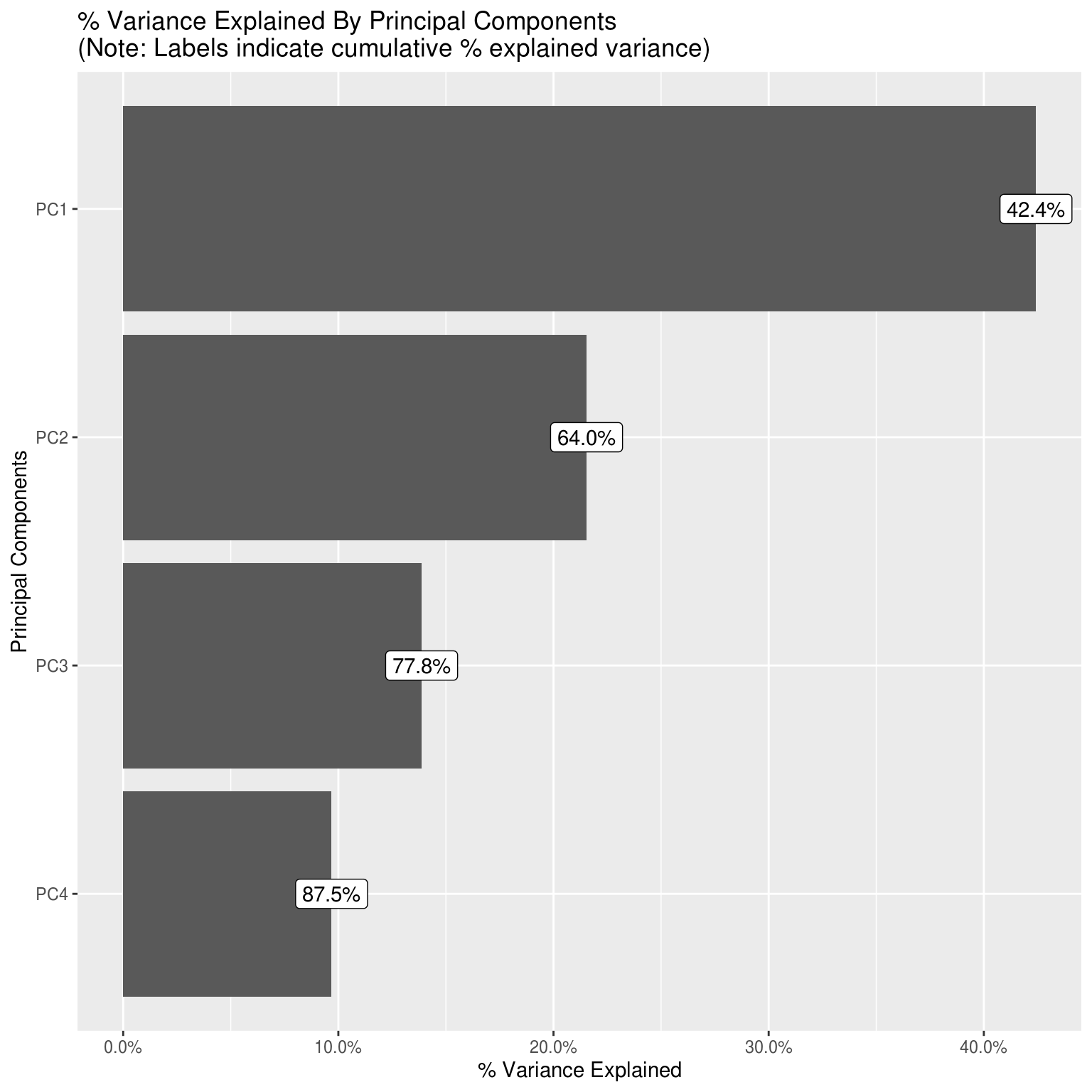
DataExplorer::plot_prcomp(pca_df, variance_cap = 0.9, nrow = 2L, ncol = 2L)

By % cases with zoonotic TB

Boxplots

## Call boxplot function
DataExplorer::plot_boxplot(pca_df, by = "tb_z_prop")

Scatterplots

DataExplorer::plot_scatterplot(pca_df, by = "tb_z_prop", sampled_rows = 1000L)