Chapter 3 getTBinR: an R package for accessing and summarising World Health Organization Tuberculosis data
3.1 Introduction
Developing tools for rapidly accessing and exploring datasets benefits the public health research community by enabling multiple datasets to be combined in a consistent manner, increasing the visibility of key datasets, and providing a framework that can be used to explore key questions of interest. Tooling also reduces the barriers to entry, allowing non-specialists to explore datasets that would otherwise be inaccessible. This widening of access may also lead to new insights and wider interest for key public health issues.
getTBinR is an R package[43] that I developed to facilitate working with the data[19] collated by the World Health Organization (WHO) on the country level epidemiology of Tuberculosis (TB). All data is freely available from the WHO5 and the package code is archived on Zenodo6 and Github7. The aim of getTBinR is to allow researchers, and other interested individuals, to quickly and easily gain access to a detailed TB dataset and to start using it to derive key insights. It provides a consistent set of tools that can be used to rapidly evaluate hypotheses on a widely used dataset before they are explored further using more complex methods or more detailed data. Prior to the development of getTBinR access to the WHO data was ad-hoc and there were no standardised visualisation or summary tools.
The remainder of this chapter outlines the structure, and key functionality, of getTBinR 0.6.1. The use of getTBinR in this thesis is explored as well as the use of the package in work external to this thesis and by others. Much of the work done for this chapter was code, documentation, and case study development and so is not fully captured here. The GitHub repository contains a full development history of the package, as well as providing links to the documentation and accompanying case studies.
3.2 Installation
getTBinR has been released to the Comprehensive R Archive Network (CRAN) and can therefore can be installed with the following code,
install.packages("getTBinR")As getTBinR is under active development, the development version can be installed from GitHub with the following,
# install.packages("remotes")
remotes::install_github("seabbs/getTBinR")
3.3 Data extraction and variable look-up
The data sourced by getBTinR is collated by the WHO, via member governments, and used to compile the yearly global TB report.[19] Data collation and estimation encompasses TB incidence, TB mortality rates, the age distribution of TB cases, the proportion of drug resistant cases, case detection rates, and treatment rates. For a complete description of the data and data collection process, see [19]. These data are used by the WHO, governmental organisations and researchers to summarise country level TB epidemiology, as well as the wider global and regional picture.
getTBinR provides a single user facing function for data extraction, get_tb_burden. This function downloads multiple datasets from the WHO, cleans variables names where required, and finally joins all datasets together. On top of the core datasets provided by default, getTBinR also supports importing multiple other datasets. These include data on latent TB, HIV surveillance, intervention budgets, and outcomes (see ?additional_datasets for a full list of available datasets). To reduce unnecessary downloads, and improve performance, downloads are cached automatically. get_tb_burden is called by all other package functions allowing for a seamless user experience. get_data_dict has similar functionality to get_tb_burden but extracts data dictionaries rather than the underlying data. It is called by the majority of the package functions in order to provide intelligent labels.
To improve the user experience, and to facilitate intelligent labeling, getTBinR provides a search function for the data dictionary (search_data_dict). This function is able to search, using fuzzy matching, for variables, variable descriptions, key phrases, and datasets. The code below gives an example search for country and e_inc_100k (TB incidence rate) variables, along with an accompanying search for variables referencing mortality.
search_data_dict(var = c("country","e_inc_100k"),
                 def = c("mortality"), verbose = FALSE)
# A tibble: 11 x 4
variable_name dataset code_list definition
<chr> <chr> <chr> <chr>
1 country Country ide… "" Country or territory name
2 e_inc_100k Estimates "" Estimated incidence (all forms…
3 e_mort_100k Estimates "" Estimated mortality of TB case…
4 e_mort_100k_hi Estimates "" Estimated mortality of TB case…
5 e_mort_100k_lo Estimates "" Estimated mortality of TB case…
6 e_mort_exc_tbhiv… Estimates "" Estimated mortality of TB case…
7 e_mort_exc_tbhiv… Estimates "" Estimated mortality of TB case…
8 e_mort_exc_tbhiv… Estimates "" Estimated mortality of TB case…
9 e_mort_tbhiv_100k Estimates "" Estimated mortality of TB case…
10 e_mort_tbhiv_100… Estimates "" Estimated mortality of TB case…
11 e_mort_tbhiv_100… Estimates "" Estimated mortality of TB case…3.4 Data visualisation
getTBInR implements a range of functions to allow rapid development of complex visuals, with minimal R knowledge. All functions make use of cached data so that no data needs to be provided and can automatically match variables to variable names. Additionally, all visualisation functions have a common user interface, allowing for knowledge transfer between functions. As all visualisation functions return ggplot2 objects (a commonly used R graphing library), user modification is readily supported.
Functionality that is common to all plotting functions is the ability to: plot data for a given list of countries; fuzzy match country names; plot data for a given metric present in the data; compute percentage changes from raw metric values; look up the supplied metric to see if the data dictionary contains an appropriate name; plot data over a user supplied range of years; facet over a user supplied variable; implement a user supplied transform (i.e log scaling); modify the colour palette used; and switch to comparable interactive graphics (using the plotly package). In addition to this, plot_tb_burden and plot_tb_burden_summary can incorporate confidence intervals. By default this is done by searching the data provided for matching variables. Function specific functionality is outlined below.
3.4.1 Mapping TB burden metrics
The map_tb_burden function makes use of an inbuilt, country level, shapefile (a geospatial vector data format) to produce a global or regional map of the metric supplied. Figure 3.1 gives a global overview of country level TB incidence rate. The use of a map here allows for the identification of spatial patterns that would be difficult to distinguish using other plot types. Figure 3.1 was produced with the following code,
map_tb_burden(metric = "e_inc_100k", verbose = FALSE) +
  theme(text = element_text(size = 12))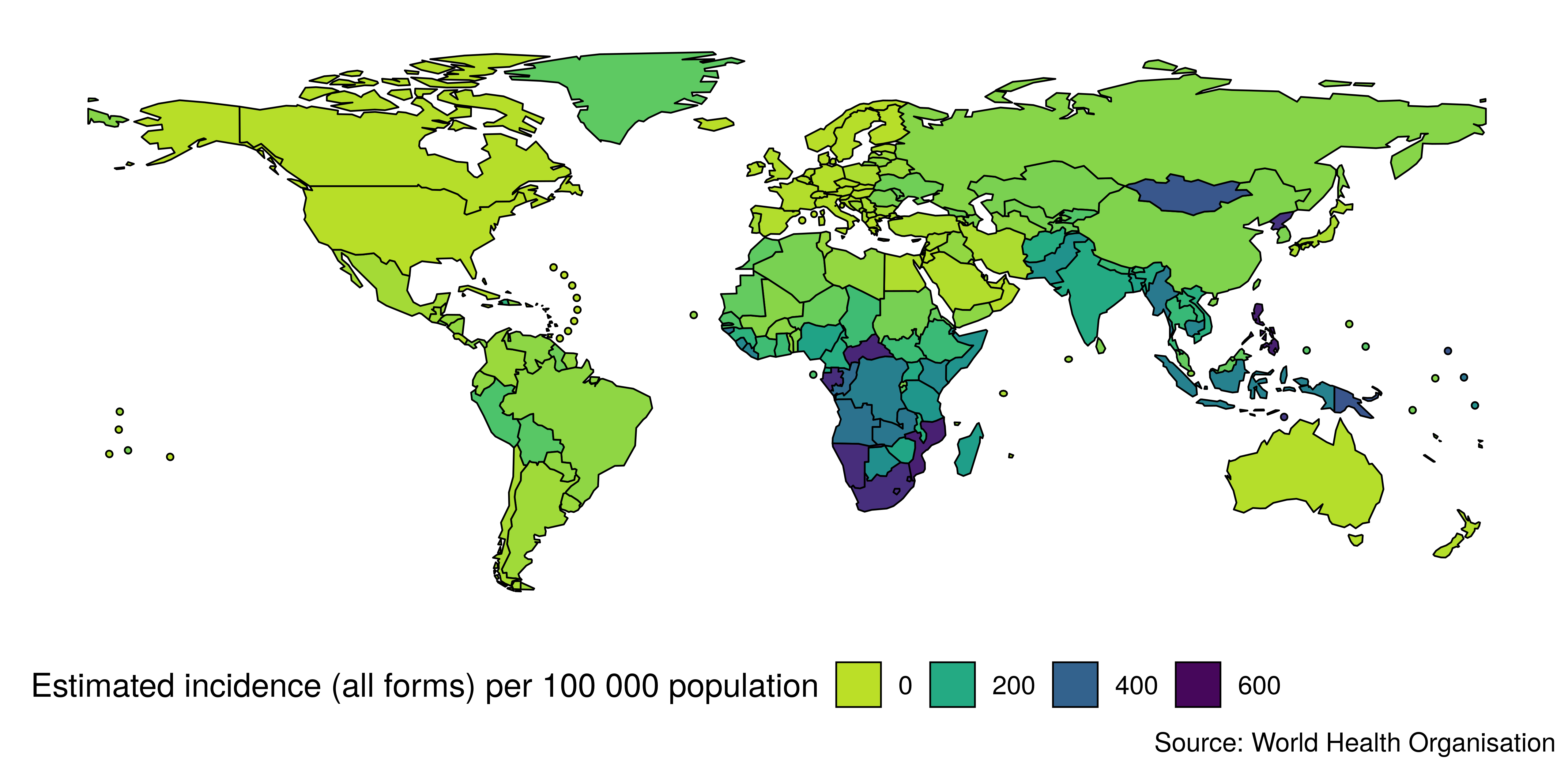
Figure 3.1: Map of global TB incidence rates in 2017 as generated by getTBinR. Visualising the data with a map allows for spatial trends to be rapidly explored.
3.4.2 Plotting an overview for a given TB metric
The plot_tb_burden_overview function returns a dot plot that allows the trend over time of a metric to be plotted in a simplified way. Figure 3.2 shows incidence rates, by country, in Europe from 2000 to 2017. The dot plot format allows us to identify common trends across countries, after ranking for incidence rate. A more traditional line plot of the same data would be difficult to interpret due to the large number of countries. Figure 3.2 was produced with the following code,
plot_tb_burden_overview(metric = "e_inc_100k",
                        countries = "United Kingdom",
                        compare_to_region = TRUE,
                        interactive = FALSE,
                        verbose = FALSE) +
  theme(text = element_text(size = 12))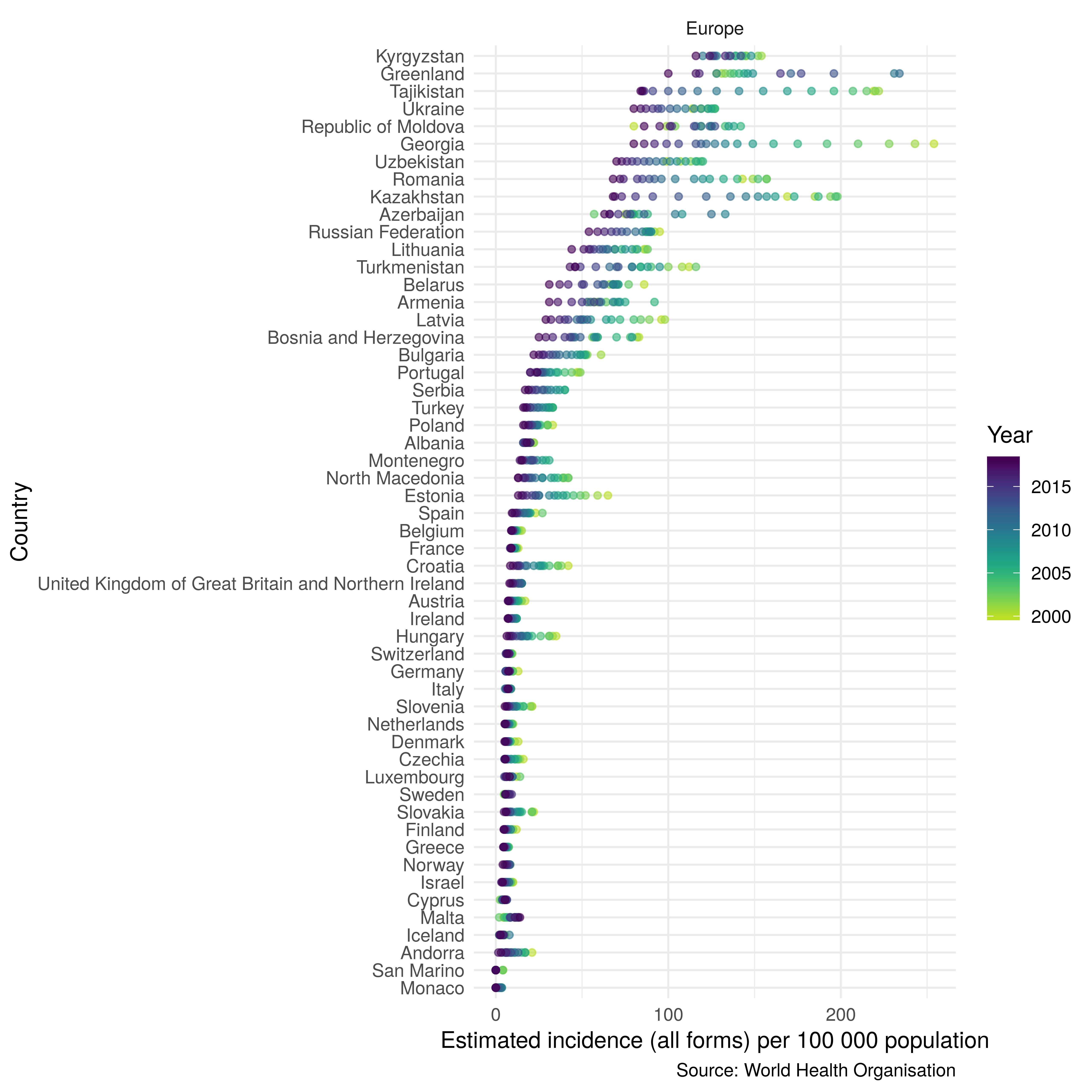
Figure 3.2: Dot plot showing trends over time in TB incidence rates in Europe ordered by TB incidence rates in 2017.
3.4.3 Plotting a comparison between country, regional and global metric values
The plot_tb_burden_summary function plots a regional, global, or custom overview of the supplied metric and can also include country level data for comparison. It can make use of a range of summary methods including: the country level mean, country level median, and summarised rates and proportions. Rates and proportions can be weighted with a user supplied variable but the package default is to use the summarised population. Confidence intervals are recomputed using a bootstrapping method where appropriate so that country level uncertainty is properly incorporated into the summarised metrics. The data can also be smoothed using a locally weighted regression to provide trend lines. Figure 3.3 shows a regional summary of TB incidence rates produced using plot_tb_burden_summary. This plot allows regional trends to be identified and compared against the global trend. Figure 3.3 was produced with the following code,
plot_tb_burden_summary(conf = NULL, metric_label = "e_inc_100k",
                       verbose = FALSE) +
  theme(text = element_text(size = 12))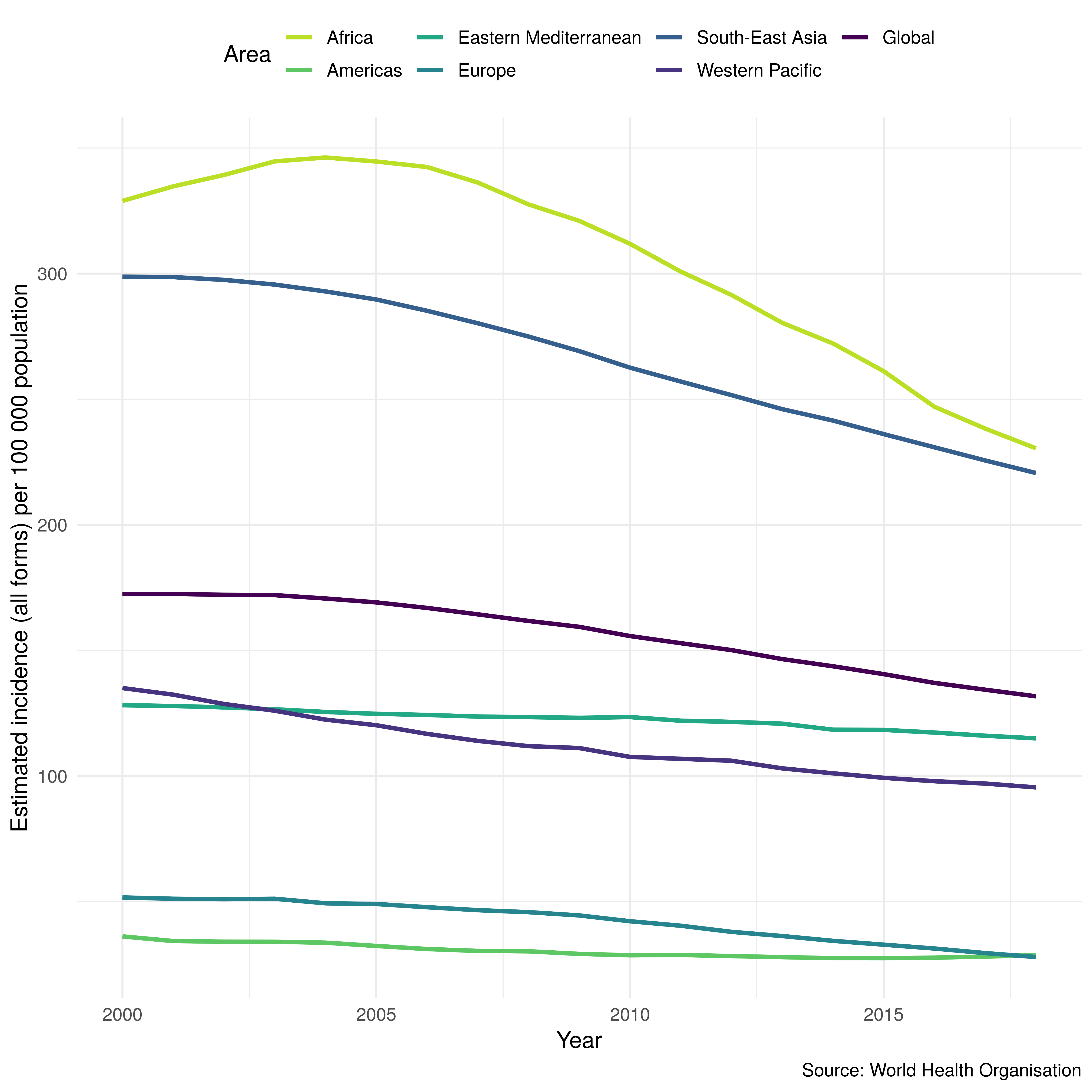
Figure 3.3: TB incidence by region and globally as computed and visualised by getTBinR. Confidence intervals have been disabled in order to avoid obscuring the dominant trends.
3.5 Plotting country level trends for a given metric
The plot_tb_burden function plots TB trends at a country level using a simple, unaggregated, line plot. This allows for trends identified with the more complex plotting functions outlined above to be examined in more detail. Figure 3.4 shows the trend over time in TB incidence rates in the United Kingdom, along with confidence intervals. Unlike the plots above the focus on a single country allows changes over time to be more easily understood. Figure 3.4 was produced with the following code,
plot_tb_burden(metric = "e_inc_100k",
               countries = "United Kingdom",
               verbose = FALSE) +
  theme(text = element_text(size = 12))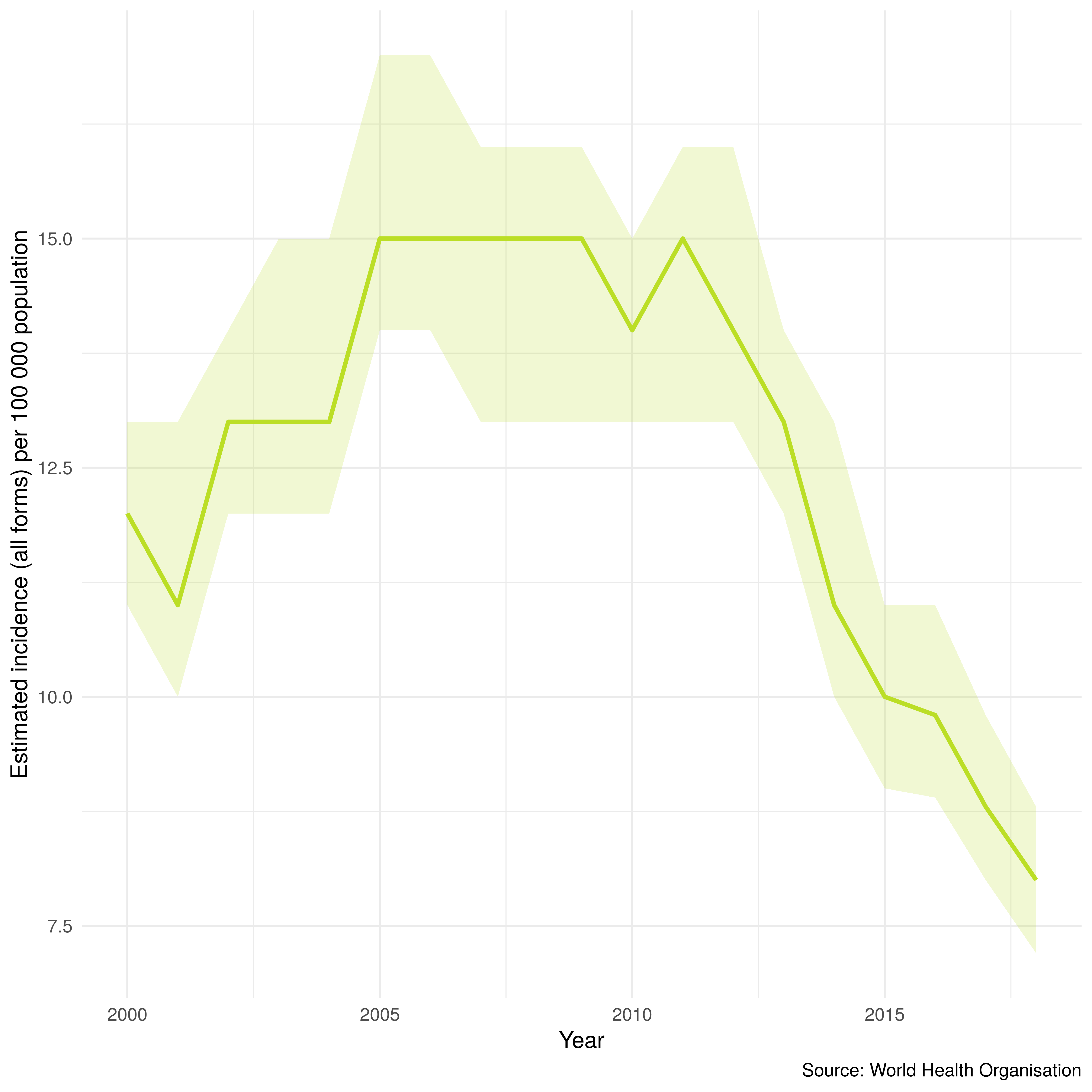
Figure 3.4: TB incidence rates over time, with confidence intervals, in the UK. As produced by getTBinR.
3.6 Data summarisation
The same summarisation functionality outlined in 3.4.3 is also available in a separate function, summarise_tb_burden, which can be used to generate summarised datasets for further analysis or visualisation. All non-plotting functions outlined for plot_tb_burden_summary are implemented here. The code below summarises TB incidence rates in the UK, in Europe, and globally.
summarise_tb_burden(metric = "e_inc_num",
                     stat = "rate",
                     countries = "United Kingdom",
                     compare_to_world = TRUE,
                     compare_to_region = TRUE,
                     verbose = FALSE)
# A tibble: 152 x 5
area year e_inc_num e_inc_num_lo e_inc_num_hi
<fct> <int> <dbl> <dbl> <dbl>
1 United Kingdom of Great Brita… 2000 11.9 10.7 13.1
2 United Kingdom of Great Brita… 2001 11.5 10.3 12.7
3 United Kingdom of Great Brita… 2002 13.1 11.8 14.3
4 United Kingdom of Great Brita… 2003 13.4 12.1 14.8
5 United Kingdom of Great Brita… 2004 13.2 11.9 14.5
6 United Kingdom of Great Brita… 2005 15.3 13.8 16.6
7 United Kingdom of Great Brita… 2006 15.3 13.8 16.4
8 United Kingdom of Great Brita… 2007 14.6 13.2 16.1
9 United Kingdom of Great Brita… 2008 15.0 13.5 16.1
10 United Kingdom of Great Brita… 2009 14.5 13.1 15.9
# … with 142 more rows3.7 Dashboard
To explore the package functionality in an interactive session, or to investigate TB without having to code extensively in R, a shiny dashboard has been built into the package. This can either be used locally using,
run_tb_dashboard()Any metric in the WHO TB data can be explored, with country selection using the built in map, and animation possible by year. The shiny app can also be used to generate the country level reports discussed in the next section. Figure 3.5 shows a screenshot of the dashboard, with South Africa selected as the country of interest.
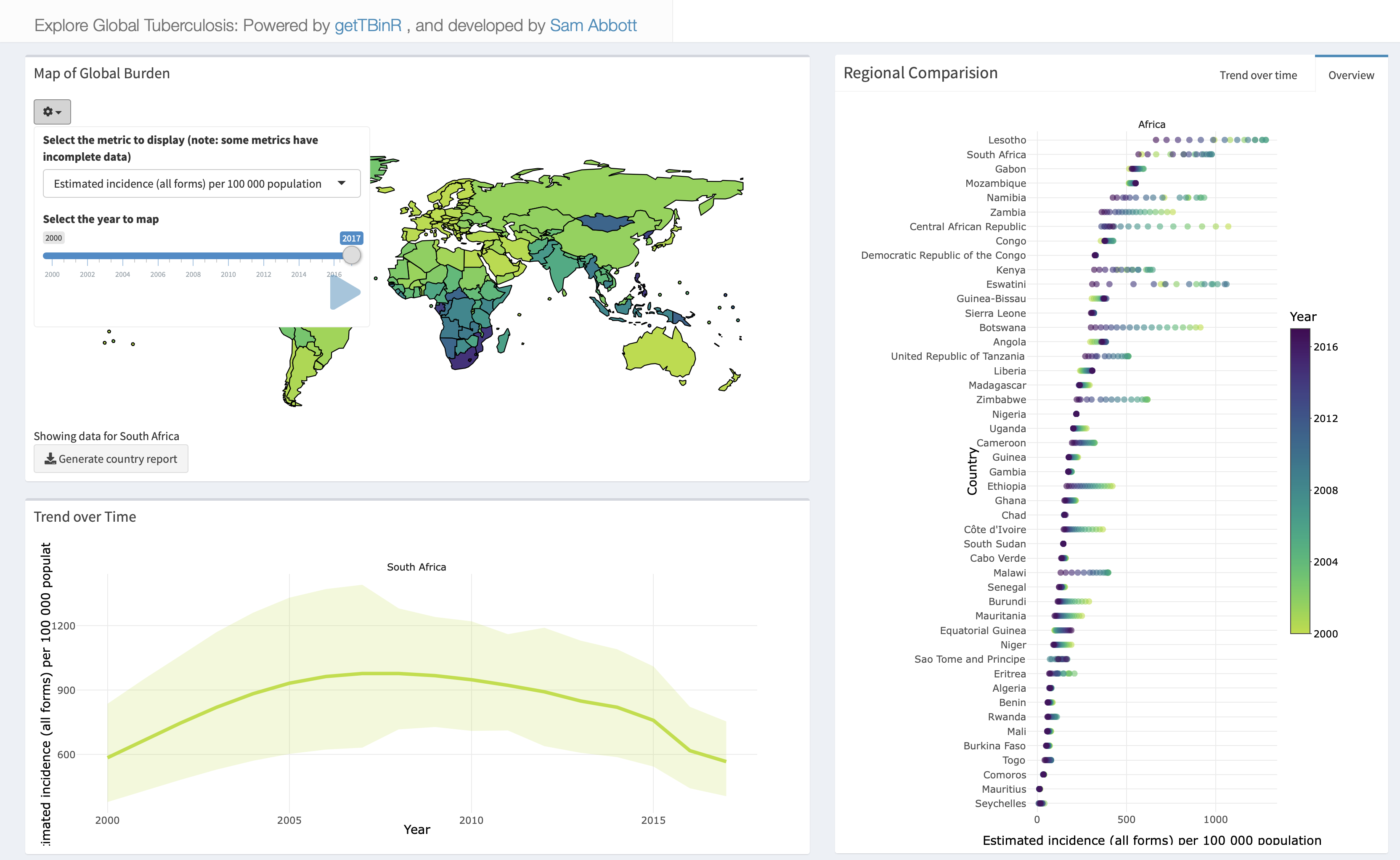
Figure 3.5: Snapshot of the built in package dashboard.
3.8 Country report
An automated country level report has also been built into getTBinR. This summarises key TB metrics and provides regional and global rankings. The most commonly required plots are also produced, including the trend in TB incidence rates, proportion of cases that lead to death, and the proportion of cases with MDR-TB. The report can be generated with the following code,
## Code saves report into your current working directory
render_country_report(country = "United Kingdom", save_dir = ".")
Figure 3.6 shows a screenshot of the start of the report for the United Kingdom. Note the automated reporting of country rankings in the text, along with summary metrics of interest.
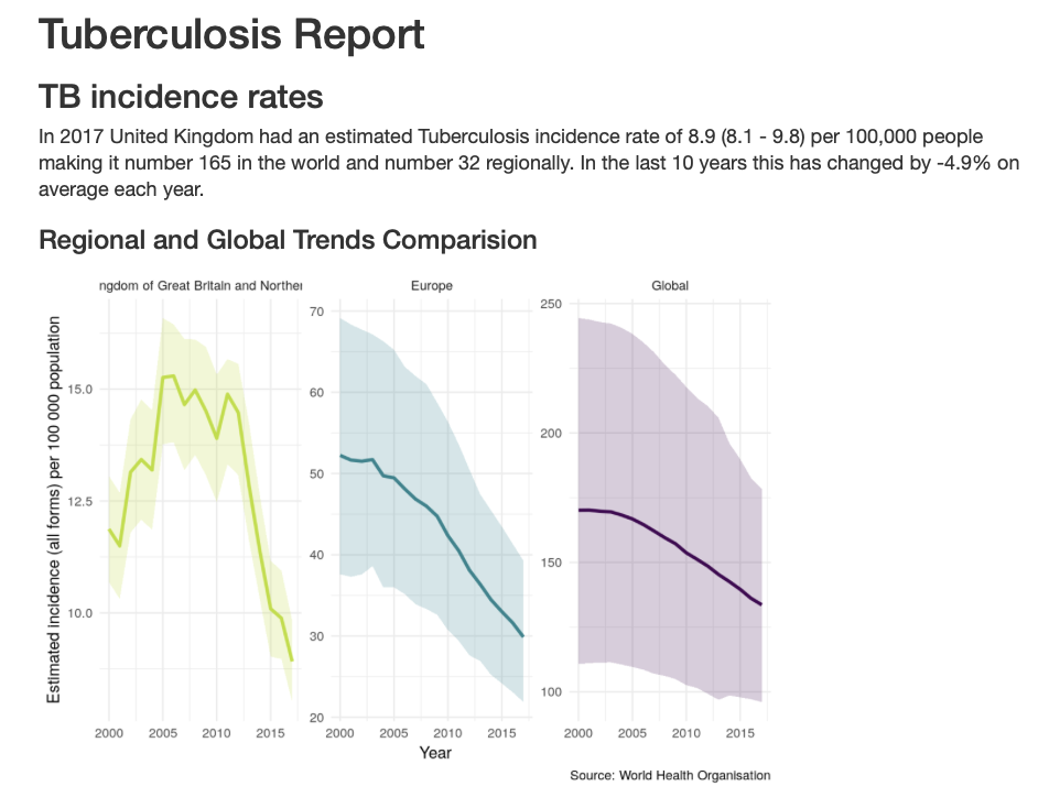
Figure 3.6: Screenshot of the start of the built-in package summary report, for the United Kingdom.
3.9 Package infrastructure
getTBinR has been developed using R package best practices and as such is thoroughly tested using an automated testing suite that runs against Linux, Windows and MacOS environments. Package documentation is supplied in a searchable website8 and a development environment can be launched with a single button press9. Use cases for the package have been outlined using multiple case studies, see the package documentation for details.
3.10 Discussion
In this chapter I have introduced the getTBinR R package. getTBinR facilitates downloading the most up-to-date version of multiple TB relevant data sources from the WHO, along with the accompanying data dictionaries. It also contains functions to allow easy exploration of the data via searching data dictionaries, summarising key metrics on a regional and global level, and visualising the data in a variety of highly customisable ways. In addition, it provides both a dashboard and an automated country level report that enables the global, regional, and country level picture to be quickly summarised. It was developed using R package development best practices and has been peer-reviewed.[44]
As of the 8th of August 2019, getTBinR has been released on CRAN for over a year. It has been downloaded over 10,000 times, has a growing user base, no outstanding bug-related issues, and has received multiple updates greatly expanding the functionality available. The standalone dashboard hosted online10 has had over 3000 unique users. It has been used as a teaching aid, as an example of open science, to facilitate exploratory data analysis and to provide context for other research. In this thesis, it has been used extensively in Chapter 2 to provide context and was also used as a hypothesis generating tool in all other chapters. Outside of the work presented in this thesis I have used getTBinR extensively as a data analysis tool11, to widen the appreciation of TB as a global health problem12, and to provide contextual information for other research13.
Whilst getTBinR is feature complete, and stable, development work continues. Future projects include: using the shinymeta R package to provide downloadable R code to users of the interactive application; iterating on the current automated report to improve formatting and to increase the amount of information displayed; and expanding the range of visualisation functions available. As additional WHO TB data are released they will be added to getTBinR.
3.11 Summary
In this chapter I have introduced
getTBinRan R package for accessing, summarising and visualising the WHO TB surveillance dataset used to compile the yearly WHO global TB report.I have outlined the need for data access packages in general - more specifically explaining the purpose of
getTBinR, detailing the package functionality and outlining the package infrastructure used.The current impact and future direction of
getTBinRhas also been detailed.
References
19 World Health Organisation. Global Tuberculosis Report. 2018.
43 R Core Team. R: a language and environment for statistical computing. 2019.
44 Abbott S. getTBinR: an R package for accessing and summarising the World Health Organisation Tuberculosis data. Journal of Open Source Software 2019;4:1260. doi:10.21105/joss.01260
WHO TB data: https://www.who.int/tb/country/data/download/en/↩
Binder: https://mybinder.org/v2/gh/seabbs/getTBinR/master?urlpath=rstudio↩
Twitter: https://twitter.com/search?q=getTBinR&src=typd; Reddit: https://www.reddit.com/user/seabbs/posts/↩
Presentation: https://www.samabbott.co.uk/what-do-we-really-know-about-bcg/presentation.html#1↩